Example 2: GLOW study
In the Global Longitudinal study of Osteoporosis in Women (GLOW), data was collected from tens of thousands of women worldwide concerning risk factors for osteoporosis, and they were followed up to determine whether they suffered a bone fracture of any kind within the subsequent year. In the logistic regression model analyzed in the text by Hosmer and Lemeshow, the objective is to predict whether a participant will suffer a fracture, based on the risk factor data. The sample consists of a subset of 500 records for participants from the U.S., and those who suffered fractures were over-sampled so that their fraction is exactly 25%, compared to an actual fraction of 4% within the larger population. The data and models for the analysis shown below can be found in this file: GLOW_logistic_models.xlsx.
The variables are FRACTURE (yes or no), PRIORFRACTURE (prior fracture, yes or no), AGE (years), WEIGHT (kilograms), HEIGHT (cm), BMI (body mass index in kg/m2), PREMENO (premenopausal, yes or no), MOMFRAC (mother had hip fracture, yes or no) ARMASSIST (arms are needed to stand from chair, yes or no) SMOKE (former or current smoker, yes or no), and RATERISK (self-reported risk of fracture relative to others of same age, on a scale from 1 to 3).
In Hosmer and Lemeshow's analysis, interactions are also considered, leading to the construction of 15 additional variables formed from pairwise products of the others. The final model includes two of these--AGExPRIORFRAC and MOMFRACxARMASSIST--as well as AGE, HEIGHT, PRIORFRAC, MOMFRAC, ARMASSIST, and RATERISK3. The same model will be demonstrated in RegressIt, along with a reformulated version of it that yields some additional insight.
First, let's look at the correlation matrix of the variables in the model:
The variables most strongly correlated with FRACTURE are AGE, AGExPRIORFRAC, and PRIORFRAC, all with correlations sllightly greater than 0.2, not large in absolute terms. (A big value of R-squared is not to be expected.) The most interesting number in the matrix is the correlation of 0.99 between PRIORFRAC and AGExPRIORFRAC. To see what is going on, let's look at series plots of these variables, with the data sorted on PRIORFRAC so that all of its zeros come first. The following pictures are obtained:
The values of AGE are all positive and bounded far away from zero relative to their range (55 to 90). The variable AGExPRIORFRAC therefore looks quite a lot like PRIORFRAC. In fact, its pattern is the same except for the addition of some noise in the string of positive values at the end, hence the very high correlation between them.
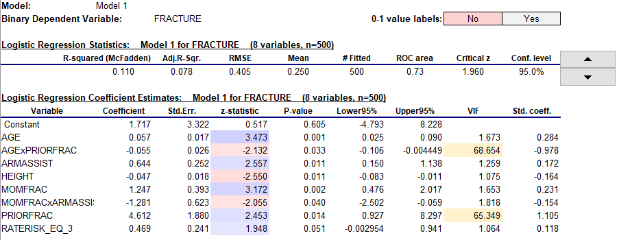
The summary statistics and coefficient table for Hosmer and Lemeshow's model are shown below. R-squared and adjusted R-squared (McFadden's version) are pretty small (0.11 and 0.078) as anticipated. The coefficient estimates are all (barely) significantly different from zero by the usual standard, with z-stats (analogous to t-stats in a linear regression model) roughly between 2.0 and 3.5 magnitude.
A red flag is waving, though: the variance inflation factors for the two highly correlated variables are in the upper 60's! Normally a VIF greater than 10 is considered as an indicator of significant multicollinearity, so this is pathological multicollinearity. An independent variable's VIF is the value of 1-divided-by-1-minus-R-squared in a linear regression of itself on the other independent variables. A VIF in the upper 60's corresponds to an R-squared of greater than 98% in such a regression, and this could have been anticipated from the correlation of 0.99 between these two variables alone. In the correlation matrix of coefficients for this model (not shown here), the correlation between the coefficient estimates for these two variables is greater than 0.99.
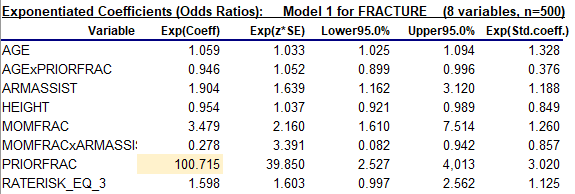
A related problem appears in the table of exponentiated coefficients: the exponentiated coefficient of PRIORFRAC is 100!
A variable's exponentiated coefficient is the factor by the which the predicted odds in favor of a positive outcome are multiplied when that variable's value is increased by one unit, holding the other variables fixed. Here this means that the predicted odds in favor of a fracture are increased by a factor of 100 by the presence of a prior fracture (i.e., by changing PRIORFRAC from 0 to 1). This seems rather surprising at first glance, given that the correlation between PRIORFRAC and FRACTURE is not very large. What's going on? The catch here is "holding the other variables fixed." Because AGE is always positive, there is no value at which AGExPRIORFRAC can be held fixed as the value of PRIORFRAC is changed from 0 to 1. It must go up by an amount that is somewhere between 55 and 90. Therefore the exponentiated coefficient of PRIORFRAC cannot be evaluated independently of the exponentiated coefficient of AGExPRIORFRAC. What one gives the other takes away.
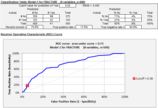
The classification table and ROC chart for the model look like this with the default cutoff value of 0.5:
The classification table and ROC chart for the model look like this with the default cutoff value of 0.5:
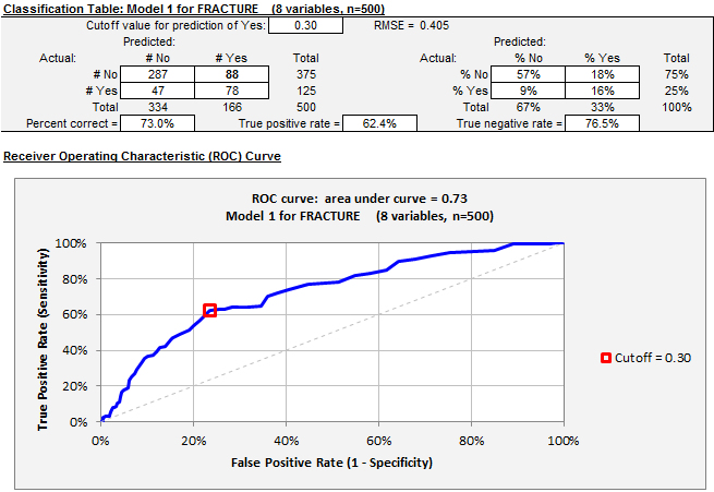
With this cutoff value, the model achieves a very low false positive rate (fraction of negative outcomes that are incorrectly predicted to be positive) but also a very low true positive rate (fraction of positive outcomes that are correctly predicted to be positive), and its position on the ROC curve is therefore down in the lower left corner of the chart. (The false positive rate is 1 minus the true negative rate.) A lower value for the cutoff level will increase the number of positive predictions, leading to an increase in the true positive rate at the expense of the false positive rate, i.e., a movement to a higher point on the curve. Here's the picture for a cutoff value of 0.3:
The percent of correct predictions has gone down very slightly (76% to 73%), and the model has achieved a very great increase in the true positive rate (18% to 62%) without nearly as great an increase in the false positive rate (5% to 23%). Whether this new cutoff value should be chosen in preference to the default value of 0.5 ought to depend on the relative consequences of error in decisions that may depend on the predictions. The ROC chart is agnostic about the cutoff level: it merely shows you the whole frontier of what is achievable.
What can be done about the multicollinearity issue? It can be addressed by constructing the interaction variables in a different but logically equivalent way in order to reduce their correlations with other variables. Here's one way to do it. First, apply a standardization transformation to AGE to convert it to units of standard deviations from its own mean. This can be done in a few seconds by using the variable transformation tool in RegressIt, yielding a new variable called AGE_STDZ. Then create two new interaction variables, one of which is PRIORFRAC times AGE_STDZ and the other of which is (1- minus PRIORFRAC) times AGE_STDZ. When these variables are plotted alongside PRIORFRAC, they look like this:
What can be done about the multicollinearity issue? It can be addressed by constructing the interaction variables in a different but logically equivalent way in order to reduce their correlations with other variables. Here's one way to do it. First, apply a standardization transformation to AGE to convert it to units of standard deviations from its own mean. This can be done in a few seconds by using the variable transformation tool in RegressIt, yielding a new variable called AGE_STDZ. Then create two new interaction variables, one of which is PRIORFRAC times AGE_STDZ and the other of which is (1- minus PRIORFRAC) times AGE_STDZ. When these variables are plotted alongside PRIORFRAC, they look like this:
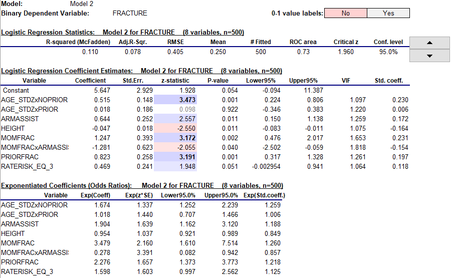
The values of the two transformed variables are now centered around zero, so that neither of them has an extremely large correlation with the other or with PRIORFRAC, and both could be feasibly fixed at zero while PRIORFRAC is hypothetically varied. Also, they are constructed in such a way as to treat the two prior-fracture conditions symmetrically, and the coefficients of the new interaction variables will be relatively independent measures of the age effect in the two different groups of women. This set of three variables is equivalent to the original set in terms of predictive capability, because the three variables in the second set can be formed from linear combinations of those in the first set, and vice versa, but they are much more useful for inference. Here is the result that is obtained when the model is re-run with the two new interaction variables used in place of AGE and AGExPRIORFAC:
The variance inflation factors are now very satisfactory and the exponentiated coefficient of PRIORFRAC no longer has a crazy value. Most interestingly, the coefficient of AGE_STDZxPRIOR is not significantly different from zero in this model (t=0.098, P=0.922). This means that age does not have predictive value concerning a bone fracture within the next year for someone who has already had a bone fracture. This is very much in line with intuition, but it did not stand out as an inference in the original model. In that model, the negative coefficient of PRIORFRACxAGE suggested that age was less of a factor for someone with a prior fracture, but not that it was statistically insignificant. Meanwhile, age does have predictive value for someone who has not yet experienced a bone fracture, as indicated by the t-stat of 3.473 (P=0.001) for AGE_STDZxNOPRIOR.
Notice that the error measures and the coefficients of all the other variables have been unchanged by this transformation of the interaction variables, reflecting the fact that the two models are logically equivalent as far as prediction is concerned.
Notice that the error measures and the coefficients of all the other variables have been unchanged by this transformation of the interaction variables, reflecting the fact that the two models are logically equivalent as far as prediction is concerned.


