Forecasting
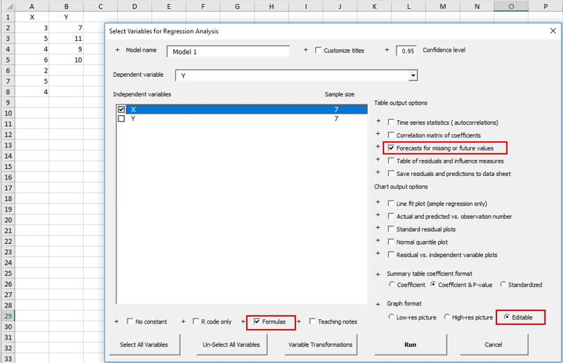
If the "Forecasts for missing or additional values" box is checked on the regression input panel, RegressIt will automatically compute forecasts for any rows in which the dependent variable is missing and the independent variables are all present. Here's an example of a simple regression model in which Y is predicted from X. The sample consists of 4 rows of data, and forecasts for Y are to be computed from 3 additional values of X. The data range consists of all 7 rows for both variables, and Y is missing in the last 3 rows.
If the "Forecasts for missing or additional values" box is checked on the regression input panel, RegressIt will automatically compute forecasts for any rows in which the dependent variable is missing and the independent variables are all present. Here's an example of a simple regression model in which Y is predicted from X. The sample consists of 4 rows of data, and forecasts for Y are to be computed from 3 additional values of X. The data range consists of all 7 rows for both variables, and Y is missing in the last 3 rows.
The output of the model includes a forecast table and chart as shown below. If the "Formulas" and "Editable charts" options are chosen, the confidence limit cells on the worksheet will contain formulas that allow the confidence level to be varied interactively via the Conf+ and Conf- buttons. You can also type a new value for the confidence level directly into cell I10, which will work even if RegressIt is not running. Try it and see! This will give you an appreciation of the meaning of "confidence" and how its value need not always be 95%. The file for this example can be found at this link.
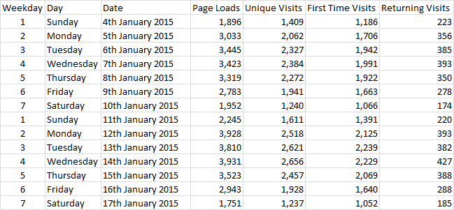
Here's a more detailed example that shows the construction of a forecasting model for a time series with a day-of-week seasonal pattern. The dataset consists of daily counts of visitors to an educational web site. Click here to download the file with the data and model. The first two weeks of data look like this:
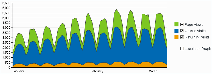
Here's a chart of the variables produced by StatCounter, the web site tracking service that collected the data. It highlights the very dramatic day-of-week effect: traffic levels are highest between Monday and Thursday, somewhat lower on Friday, and much lower on Saturday and Sunday.
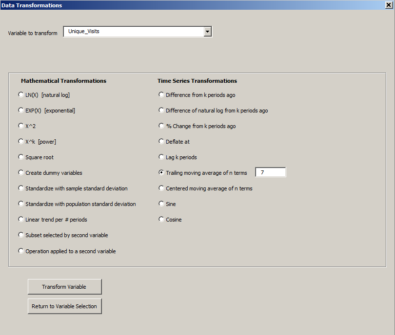
For purposes of demonstration, a regression model will be used to predict the Unique Visits series (i.e., the number of different visitors on a given day). A 7-day trailing moving average is first computed in order to determine the local average daily level of unique visits. This can be done with the variable transformation tool in RegressIt:
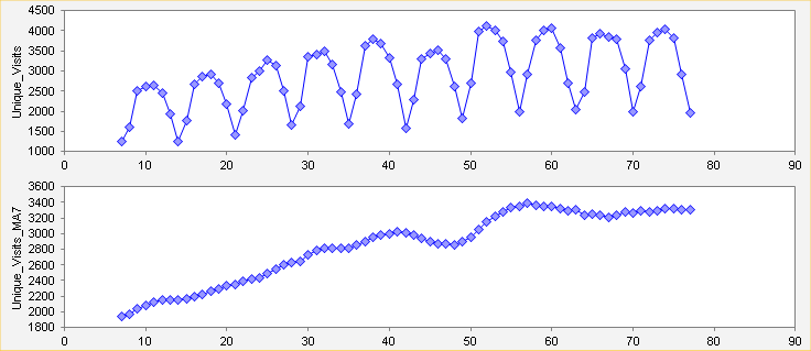
Series plots of the unique visitors series and its 7-day moving average produced by the Data Analysis procedure are shown below. The moving average completely smooths out the day-of-week effect. There is a strong annual seasonal pattern in this series, which is keyed to the academic calendar and the occurrence of major holidays. Here we see that there was steady upward growth in the first half of the series, early in the Spring semester. Activity typically levels off in the second half of the semester and then jumps upward at the very end before dropping to a much lower level during summer vacation. An unusual dip in the pattern occurred between February 14 and February 20 (day 42 to day 48 in the sample ), which was due to the disruption of business and school activity in the Eastern U.S. by a series of winter storms that hit over the period from February 11 to 17.
In the model that will be fitted to this series, the forecast for a given day is equal to a multiple of the value of the trailing moving average that was observed one week ago plus an additive adjustment for the day of the week. The 1-week-ago value of the moving average is used so that the model will be capable of forecasting one week into the future. This is not the only possible model that could be used for this purpose, nor is the best for predicting what will happen at horizons of less than 7 days. (In this particular data set, it fails to respond to the sudden change in the pattern caused by the February storm.) However, it provides an illustration of one method by which a regression model can make predictions more than one period ahead. See the bottom of this page for more comments.
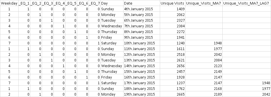
To set up this model, the moving average series is lagged by 7 periods (by using the variable transformation tool again to apply the lag transformation), and dummy variables are created for days of the week (again using the variable transformation tool). The worksheet with the transformed variables looks like this:
To set up this model, the moving average series is lagged by 7 periods (by using the variable transformation tool again to apply the lag transformation), and dummy variables are created for days of the week (again using the variable transformation tool). The worksheet with the transformed variables looks like this:
Unique_Visits_MA7 is the name of the 7-week trailing moving average variable. Its value of 1948 on January 10 is the average of the values for January 4 to January 10 (and so on). Unique_Visits_MA7_LAG7 is the moving average series lagged by 7 days, so it has a value of 1948 in the row for Saturday, January 17 (and so on). The dummy variables for the values of Weekday are shown at the left. Their names haven been partly hidden to keep the column widths narrow for display: the full title of the "_EQ_1" column is "Weekday_EQ_1", which is the name of the dummy variable for day 1 of the week (Sunday) that was created automatically by RegressIt. Its value is 1 in every Sunday row and zero elsewhere, and similarly for the dummies for other weekdays.
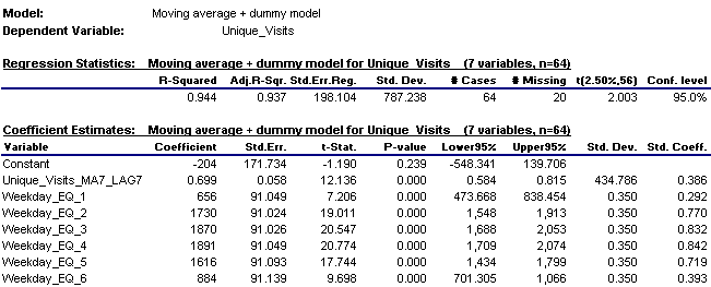
If a constant is included in the model, only 6 out of the 7 dummy variables can be used. Here are the results of fitting a model with the lagged moving average variable, dummies for the first 6 days of the week, and a constant. Adjusted R-squared is very high (94%) because the model does a very good job of explaining the dramatic and very consistent day-of-week pattern as well as adapting to week-to-week changes in the average level of the series.
If a constant is included in the model, only 6 out of the 7 dummy variables can be used. Here are the results of fitting a model with the lagged moving average variable, dummies for the first 6 days of the week, and a constant. Adjusted R-squared is very high (94%) because the model does a very good job of explaining the dramatic and very consistent day-of-week pattern as well as adapting to week-to-week changes in the average level of the series.
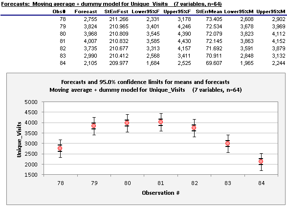
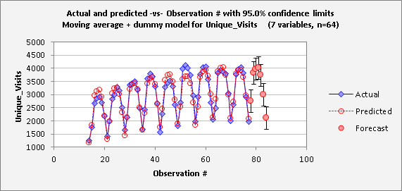
Because the moving average series has been lagged by 7 days, and because the values of the dummy variables are known in advance for any day in the future, this model is capable of forecasting 7 days ahead, and it will do so automatically if the forecasting box has been checked. Here are the forecast table and chart that RegressIt generates for the model. They include not only the point forecasts but also confidence limits for means and forecasts. (A confidence interval for the mean is a confidence interval for the location of the true regression line at a given point. A confidence interval for a forecast takes into account both the uncertainty in the location of the regression line and the unexplained variance in the data.) The confidence limits in the table and chart are calculated with live formulas: if the confidence level in cell I10 on the worksheet is changed, the limits shown in the table and chart will be instantly updated.
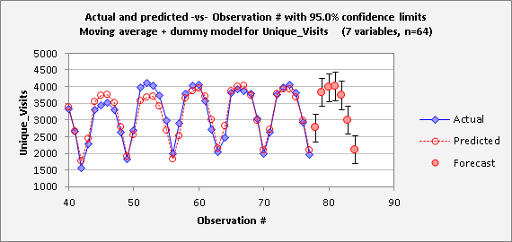
The actual-and-prediicted-vs-observation-number plot also shows the forecasts and their confidence intervals if the forecast table is currently being displayed (i.e., if it has not been not hidden). It can be seen here that the pattern in the forecasts does very closely match the day-of-week pattern in the historical data.
Here's an enlargement of the second half of the series, which gives a better look at the forecasts:
Although this model generates forecasts for the next 7 days, only the 7-day-ahead forecast makes efficient use of the past data. Each of the forecasts shown above is based on data that has been lagged by 7 days relative to its own date, but a 1-day-ahead forecast really only needs to lag the past data by 1 day, a 2-day-ahead forecast only needs to lag it by 2 days, and so on. If it is desired to have as-accurate-as-possible individual forecasts for each of the next 7 days, it is better for them to be produced by separate regression models, each of which lags the data by no more days than necessary. (For shorter horizons, it also helps to include the most recent single-day value as well as the most recent 1-week moving average.) It is easy to use RegressIt to construct separate models in which the variables are lagged by different numbers of periods and to pull out the longest-horizon forecast from the forecast table for each one. It only takes a couple of minutes to create the extra lagged variables and run the models, each of which is a minor variation on the one before it. When this is done, the results turn out to compare very favorably with what is obtained from other types of forecasting models that provide a more integrated approach to long-horizon forecasting, e.g., exponential smoothing and ARIMA models.
Click here to proceed to the Download-software page.
Click here to proceed to the Download-software page.

