Excel to R
RegressIt allows Excel to serve as a front end for running models in R and/or as a back end for producing interactive, presentation quality output on a spreadsheet after running a model in R. The steps shown below require only a small number of mouse clicks and keystrokes. The example used here is the "auto mpg" data set that is widely used in demonstrating regression and machine learning techniques. It was originally released in the 1983 ASA Data Expo, and it can now be found in many places on the internet such as: https://archive.ics.uci.edu/ml/datasets/auto+mpg. The file contains complete data for 392 cars that were sold in the U.S. between 1970 and 1982. The objective of the analysis is to predict their fuel economy from various physical attributes. An accompanying Excel file (AutoMPG_R_models.xlsx) contains an analysis of this data set in RegressIt with extensive commentary as well as an illustration of output options. This page and the next one will show how the data can be exported to R and analyzed there and how the specification of a model in R can be imported back to Excel for further analysis. A discussion of the same example can be found in this pdf file. All of the steps shown below (starting from the picture of the spreadsheet with raw data) can be carried out in a minute or two as demonstrated in the video.
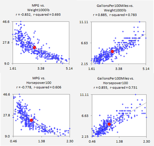
The variables to be used in the analysis have undergone some renaming and rescaling to make the modeling results easier to interpret and present, as discussed in this set of slides: DataPreparationAutoMPG.pdf. In the original file, the measure of fuel economy that is given is miles-per-gallon, and most if not all of the analyses that you will find on the internet use that as the dependent variable in the regressions. One of the modeling issues that then arises is that it is a nonlinear function of the quantitative predictor variables, which stands out clearly in scatterplots, and the usual solution is to include higher-order terms such as horsepower squared at a cost in complexity and intuition. (See this article and this book, pages 90-93 and 190-197, and sites which refer to it. Caution: it's a 12MB download of a whole book on statistical learning.) In analyses presented here, the nonlinearities will be addressed via a nonlinear transformation of the dependent variable, namely a conversion of miles per gallon to gallons-per-100-miles. In the metric world, fuel economy is similarly measured in units of liters per 100 kilometers. It is plausible that the amount of fuel required to travel a given distance should vary linearly with measures of the physical size of a car. Moving a car that is twice as big is like moving two cars. Indeed, this transformation nicely linearizes the patterns that are seen in scatterplots of the dependent variable versus the key predictors. Here is a comparison of scatterplots (produced by RegressIt) of the two fuel economy measures versus weight and horsepower, which turn out to be the most significant variables in the regressions.
(As an aside: a log transformation of all three variables produces nearly identical error stats in real units and better residual diagnostics in the units fitted, hence better calibrated confidence intervals for predictions. It also finesses the issue of whether to start from MPG or its reciprocal, because the log of one is minus the log of the other. On the margin it assumes a linear relationship in percentage units.)
In our analysis, several variables have also been rescaled so that a 1-unit change is a meaningful difference and/or they have renamed to be more self-descriptive, other aids to thoughtful modeling and communication. For example, one of the original variables is called "acceleration" and the documentation of the data set does not give its units. Further research and inspection of the data reveals that it is not a measure of the rate of change of velocity but rather its reciprocal, the elapsed time to go from 0 to 60mph, and that's how it has been labeled here.
One more issue is the treatment of the variable in the data set that is a numeric code for country of origin: 1=US, 2=Europe, 3=Japan. In some analyses of this data set that you will find, this is directly used as an independent variable in the regressions, despite the fact that no a priori justification for the ordering is given. This variable does have a strong negative correlation with gallons-per-100-miles (-0.533), which seems to make it a good candidate for a predictor. But not so fast! The effect could be due to differences in average sizes of cars produced in different countries, and indeed European cars tend to be heavier than those from Japan, and weight is even more strongly negatively correlated with the origin code, as these scatterplots show:
In the context of a multiple regression analysis, the question is how fuel economy depends on country of origin after controlling for other variables. Here, dummy variables have been created for the country codes to address this issue, and it turns out that the country effect places Japan in between the US and Europe, ceteris paribus, contrary to the ordering of their codes. Another issue that arises here is whether one of the dummies ought to be removed if its coefficient is not significantly different from zero by the usual standard. A case can be made that you should include the matched set, rather than pick and choose, otherwise you are imposing an assumption of zero difference between some pairs.
The top of the original data spreadsheet is shown below. It also includes a dummy variable for years up to 1981, called Year70To81, which will be used to designate a training set to be used for out-of-sample validation. A truncated version of the GallonsPer100Miles variable, which extends only to the end of 1981, is also included. This is needed for holding out the last year of data when running the models in Excel. The screen has been split in the picture below so that the behavior of these variables around the boundary between 1981 and 1982 can be seen.
The top of the original data spreadsheet is shown below. It also includes a dummy variable for years up to 1981, called Year70To81, which will be used to designate a training set to be used for out-of-sample validation. A truncated version of the GallonsPer100Miles variable, which extends only to the end of 1981, is also included. This is needed for holding out the last year of data when running the models in Excel. The screen has been split in the picture below so that the behavior of these variables around the boundary between 1981 and 1982 can be seen.
If your data has not already been transferred to R, the Export Data tool on the ribbon can be used export the entire contents of the data worksheet to a CSV file (a text file in comma-delimited format), At the same time, R code for reading the data from the file into a new data frame will be copied to the clipboard. The screen shots below illustrate the sequence. After Export Data is clicked, the write-data-to-text-file dialog box appears. A default file location (current folder) and file name (current data worksheet name) are offered, but they can be edited. After you hit Create File, a message box pops up to show what the exported data will look like, so you can review it.
After clicking OK you just need to go to the command prompt in RStudio and hit <Paste><Enter> in order to run the code and load the data into a new frame with same name as the file name.
Now go back to RegressIt and click the Linear Regression button on the ribbon to open the dialog box for specifying a regression model. Here GallonsPer100Miles has been selected as the dependent variable, and all other variables (except MPG) have been selected as independent variables.
If the R-code-only box is checked, the model will not be fitted in RegressIt when you hit Run. Instead you will go straight to the dialog box for choosing options for the outputs and type of modeling that you want to use in R. You can choose from an array of table and chart output, you can optionally choose forward or backward stepwise variable selection, and you can choose from a variety of options for fitting models to subsets of the data and doing out-of-sample testing. Here forward stepwise selection has been chosen. This is not an endorsement of stepwise regression, just a demonstration of available options, and it is rather silly to use any sort of automatic variable selection method for fishing in such a small pool of variables.
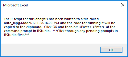
When you hit the Run button in this dialog box, two things will happen. The code for running the analysis will be written to an R script file (whose extension is .r), and the code for reading and executing the script will be written to the clipboard. A message box with this information will pop up as pictured below. If you run many models in your session, you will have an audit trail of script files, and these can be re-run at any later time to replicate the results. The script files have uniquely identifying default names of the form dataframe.modelname.month.day.hour.minute.second, but you can customize them. You can also customize the location for the script files.
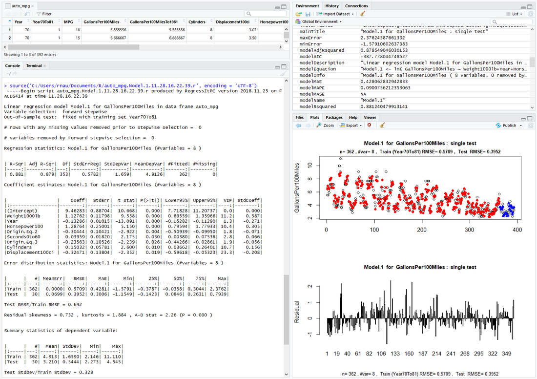
A line of R code with a source(.) command, which will execute the script, is written to the clipboard. Just go to the command prompt in RStudio and hit <Paste><Enter> to run it. In this case the table and output below will be produced in the various panes in RStudio.
The forward stepwise selection option has not removed any variables, as it turns out, and the t-stats of the variables are all greater than 2 in magnitude. However, a problem is apparent. Some of the variables have extremely large variance inflation factors, particularly Displacement100ci, whose VIF is 23.3. Also, its coefficient has a counterintuitive negative sign. These are signs of multicollinearity, and it's not surprising because weight, horsepower, acceleration, displacement, and number of cylinders are all positively related to the size of the car and its engine.
The two currently-visible charts are customized charts created within the script: actual and predicted values versus row number and residuals versus row number. In the first one, the red dots are fitted values and the blue triangles are out-of-sample predictions. These two charts are especially useful if the variables are time series or otherwise sorted in a meaningful way. Here the rows are sorted in blocks by year, so the forecasts for 1982 cars appear at the end.
Standard chart output was requested for this model, produced by the R's plot(.) command, yielding the 2x2 array shown below.
Go on to the next page: R to Excel.


